In what follows I'll try to explain my basic understanding and interepretation of the semi-supervised framework based on Variational Autoencoders, as described in [1]. I shall assume a vector notation where bold symbols $\mathbf{a}$ represent vectors, whose $j$-th component can be represented as $a_j$.
The starting point of the framework is to consider a dataset \(D = S \cup U\), where:
- \(S = \{(\mathbf{x}_1, \mathbf{y}_1), \ldots, (\mathbf{x}_n, \mathbf{y}_n)\}\),
- \(U = \{\mathbf{x}_{n+1}, \ldots, \mathbf{x}_{n+m}\}\),
with \(\mathbf{x}_i \in \mathbb{R}^N\) and \(\mathbf{y}_i \in \{0,1\}^C\) represents a one-hot encoding of a class in \(\{1, \ldots, C\}\).
The basic assumption of variational autoencoders is that data is generated according to a density function \(p_\theta(\mathbf{x}| \mathbf{z})\), where \(\mathbf{z}\in \mathbb{R}^K\) is a latent variables governing the distribution of \(\mathbf{x}\). \(\theta\) represents a model parameter. The above density function can be modeled through a Neural network: thus \(\theta\) represents all the network weights. An example PyTorch snippet, where the density is be modeled as a softmax over a simple linear layer, is illustrated below.
import torch
import torch.nn as nn

class Decoder(nn.Module):
    def __init__(self, latent_size,num_classes,out_size):
        super(Decoder, self).__init__()

        self.linear_layer = nn.Linear(latent_size + num_classes, out_size)
        nn.init.xavier_normal_(self.layer.weight)

        self.activation = nn.Sigmoid(dim=-1)

    def forward(self, z):
      	return self.activation(self.linear_layer(z))
Here, we are assuming $\mathbf{x}$ binary and consequently the reconstruction exploits a bernoullian distribution for each feature.
Let's see how the generative framework can model the likelihood of the data and help us develop a semi-supervised classifier.
Unsupervised examples
First, let us consider \(\mathbf{x}\in U\). When \(\mathbf{y}\) is unknown, we can consider it as a latent variable as well. Both \(\mathbf{y}\) and \(\mathbf{z}\) assume a prior distribution, given by
\[\begin{split} \mathbf{z} \sim & \mathcal{N}(\mathbf{0},I_K)\\ \mathbf{y} \sim & \mathit{Cat}(\boldsymbol\pi) \end{split}\]
Here, \(\boldsymbol\pi\) is a prior multinomial distribution over \(\{1, \ldots, C\}\).
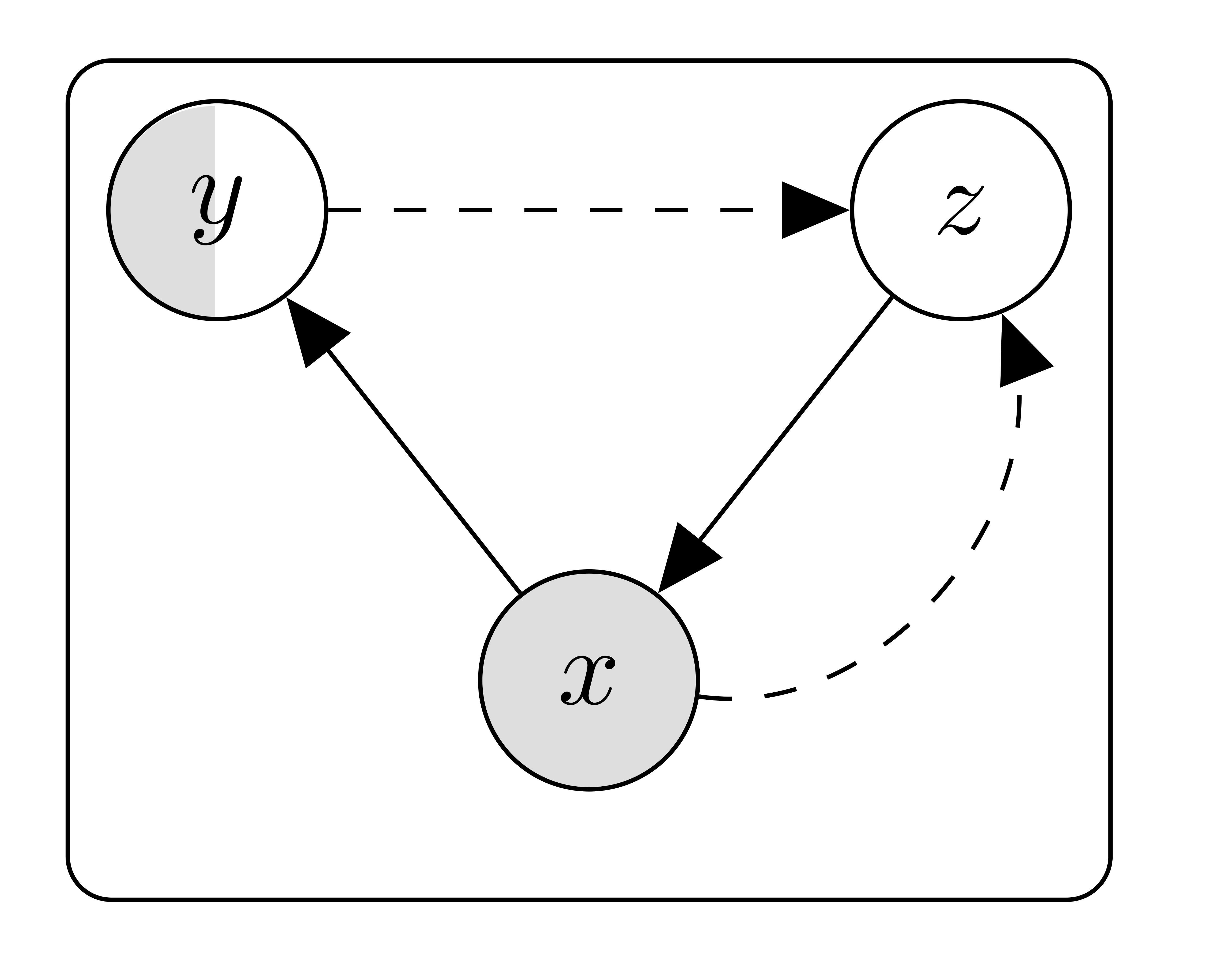
In such a case, we can extend the generative setting where data samples $\mathbf{x}$ are assumed to be generated by the conditional \(p_\theta(\mathbf{x}| \mathbf{z},\mathbf{y})\) through the relationship
\[ \begin{equation}\label{average}\tag{1} p(\mathbf{x}) = \int p_\theta(\mathbf{x}| \mathbf{z}, \mathbf{y}) p(\mathbf{z})p(\mathbf{y}) \mathrm{d} \mathbf{z} \mathrm{d} \mathbf{y} \end{equation} \]
In principle, the \(\theta\) parameter can be chosen to maximize the evidence on \(D\), i.e. by optimizing \(\log p(\mathbf{x})\). However, this approach is not feasible because it requires averaging over all possible \(\mathbf{z}\) pairs. We can approximate the likelihood by sampling a subset of $\mathbf{z}$ latent data points and then averaging over them. Again, this workaround exhibits the drawback that pure random sampling is exposed to high variance. The idea of Variational Autoencoders is to "guide" the sampling by exploiting the evidence: instead of freely choosing $\mathbf{z},\mathbf{y}$, we build a sampler \(q_\phi(\mathbf{z},\mathbf{y}|\mathbf{x})\) that tunes the probability of \(\mathbf{z},\mathbf{y}\) according to $\mathbf{x}$. In practice, $q_\phi$ encodes the information regarding \(\mathbf{x}\) into the most probable \(\mathbf{z},\mathbf{y}\) latent variables.
We can factorize the decoder as \(q_\phi(\mathbf{z},\mathbf{y}| \mathbf{x}) = q_\varphi(\mathbf{z}|\mathbf{x},\mathbf{y})q_\vartheta(\mathbf{y}|\mathbf{x})\), where
\[\begin{split} q_\varphi(\mathbf{z}|\mathbf{x},\mathbf{y}) \equiv & \mathcal{N}(\mathbf{z}| \boldsymbol\mu_\varphi(\mathbf{x},\mathbf{y}), \boldsymbol\sigma_\varphi(\mathbf{x},\mathbf{y})\cdot I_K)\\ q_\vartheta(\mathbf{y}|\mathbf{x}) \equiv & \mathit{Cat}(\mathbf{y}|\boldsymbol\pi_\vartheta(\mathbf{x})), \end{split}\]
Here, the parameters \(\boldsymbol\mu_\varphi(\mathbf{x},\mathbf{y}), \boldsymbol\sigma_\varphi(\mathbf{x},\mathbf{y})\) and \(\boldsymbol\pi_\vartheta(\mathbf{x})\) represent neural functions parameterized by $\varphi$ and $\vartheta$, respectively. Again, a PyTorch snippet is given below, where the two encoders are exemplified. Concerning \(q_\varphi(\mathbf{z}|\mathbf{x}, \mathbf{y})\), we have:
class Encoder_z(nn.Module):
def __init__(self, input_size,latent_size):
super(Decoder, self).__init__()
self.latent_size = latent_size
self.linear_layer = nn.Linear(input_size, 2*latent_size)
nn.init.xavier_normal_(self.linear_layer.weight)
def _sample_latent(self, mu_q, logvar_q):
var_q = torch.exp(logvar_q)
epsilon = torch.randn(var_q.size(),requires_grad=False).to(var_q.device)
return mu_q + epsilon*var_q
def forward(self, x, y):
input = torch.cat([x,y],dim=-1)
temp_out = self.linear_layer(input)
mu_q = temp_out[:, :self.latent_size]
logvar_q = temp_out[:, self.latent_size:]
z = self._sample_latent(mu_q, logvar_q)
return z, mu_q, logvar_q
```
The computation within this class is a variable \(\mathbf{z}\sim q_\varphi(\cdot |\mathbf{x},\mathbf{y})\), as well as the parameters of the variational (gaussian) distribution \(\boldsymbol\mu\) and \(\boldsymbol\sigma\). Here, we are exploiting the reparameterization trick: given a variable \(\boldsymbol\epsilon \sim \mathcal{N}(\mathbf{0},I_K)\), the transformation \(z = \mu + \epsilon \cdot \sigma\) guarantees that \(\mathbf{z}\sim \mathcal{N}(\boldsymbol\mu, \boldsymbol\sigma)\) and at the same time it preserves the backpropagation of the gradient, since \( \frac{\partial \mathbf{z}}{\partial w} = \frac{\partial \boldsymbol\mu}{\partial w} + \boldsymbol\epsilon \cdot \frac{\partial \boldsymbol\sigma}{\partial w} \) and both \(\boldsymbol\mu\) and \(\boldsymbol\sigma\) are deterministically computed as shown above.
Similarly, \(q_\vartheta(\mathbf{y}|\mathbf{x})\) is exemplified by the following snippet:
class Classifier(nn.Module):
    def __init__(self, input_size,num_classes):
        super(Decoder, self).__init__()

        self.linear_layer = nn.Linear(input_size, 2*latent_size)
        nn.init.xavier_normal_(self.layer.weight)

        self.softmax = nn.Softmax(dim=-1)

    def forward(self, x):
        return self.softmax(self.linear_layer(x))
Notice that, differently from the previous case, within this class we directly output a probability distribution \(q_\vartheta(\mathbf{y}|\mathbf{x})\), rather than a sample \(\mathbf{y} \sim q_\vartheta(\cdot|\mathbf{x})\). The reason for this choice is that no reparameterization trick is possible for a discrete distribution that preserves backpropagation. However, this does not prevent us from averaging over all possible samples, as we shall see later.
What is the relationship between the encoders and the decoder? We can observe that
\( \begin{split} \log p(\mathbf{x}) \geq & \mathbb{E}_{q_\phi(\mathbf{z},\mathbf{y}| \mathbf{x})}\left[\log p_\theta(\mathbf{x}| \mathbf{z}) + \log p(\mathbf{z}) + \log p(\mathbf{y}) - \log q_\phi(\mathbf{z},\mathbf{y}| \mathbf{x})\right] \\ = & \sum_\mathbf{y} \mathbb{E}_{q_\varphi(\mathbf{z}| \mathbf{x},\mathbf{y})}\Bigg[ q_\vartheta(\mathbf{y}| \mathbf{x})\bigg(\log p_\theta(\mathbf{x}| \mathbf{z}) + \log p(\mathbf{y}) - \log q_\vartheta(\mathbf{y}| \mathbf{x})\bigg) \\ & \qquad \qquad + \log p(\mathbf{z}) - \log q_\varphi(\mathbf{z}| \mathbf{x},\mathbf{y})\Bigg] \end{split} \) We call the right-hand side of the equation the Evidence Lower Bound (ELBO). It turns out that, optimizing this equation with respect to \(\phi, \theta\) corresponds to optimizing \(\log p(\mathbf{x})\) as well. Thus, we can specify the loss \(\ell(\mathit{x})\) as the negative of the ELBO and exploit a gradient-based optimization strategy. The main difference with respect to directly optimizing eq. (\(\ref{average}\)) is that the ELBO is tractable. In fact, we can rewrite it as
\(\begin{split}
\ell(\mathbf{x})= & - \sum_\mathbf{y} \mathbb{E}_{\boldsymbol\epsilon\sim \mathcal{N}(\mathbf{0},I_K)}\Bigg[ q_\vartheta(\mathbf{y}| \mathbf{x})\bigg(\log p_\theta(\mathbf{x}| \mathbf{z}(\boldsymbol\epsilon, \mathbf{x},\mathbf{y})) + \log p(\mathbf{y}) - \log q_\vartheta(\mathbf{y}| \mathbf{x})\bigg) \\
& \qquad \qquad + \log p(\mathbf{z}(\boldsymbol\epsilon, \mathbf{x},\mathbf{y})) - \log q_\varphi(\mathbf{z}(\boldsymbol\epsilon, \mathbf{x},\mathbf{y})| \mathbf{x},\mathbf{y})\Bigg]
\end{split}\)
where \(\mathbf{z}(\boldsymbol\epsilon, \mathbf{x},\mathbf{y}) = \boldsymbol\mu_\varphi(\mathbf{x},\mathbf{y}) + \boldsymbol\epsilon \cdot \sigma_\varphi(\mathbf{x},\mathbf{y})\) represents the \(\mathbf{z}\) component in the output of Decoder_z and
\(q_{\vartheta}(\mathbf{y}| \mathbf{x})\) represents the output of Classifier.
By analysing the above equation we can observe the following:
Since \(q_\vartheta(\mathbf{y}| \mathbf{x}) = \prod_{j=1}^C \pi_{\vartheta,j}(\mathbf{x})^{y_j}\) and \(\mathbf{y}\) ranges over all possible classes, we can simplify the first part of the right-hand side of the equation with \(\sum_{j = 1}^C \pi_{\vartheta,j}(\mathbf{x})\bigg(p_\theta(\mathbf{x}| \mathbf{z}(\epsilon,\mathbf{x},\mathbf{y}), \mathbf{e}_j) + \log \pi_j - \log \pi_{\vartheta,j}(\mathbf{x})\bigg)\), where \(\mathbf{e}_j\) is the vector of all zeros except for position \(j\) and \(\pi_{\vartheta,j}(\mathbf{x})\) is the \(j\)-th component of \(\pi_{\vartheta}(\mathbf{x})\).
Further, by exploiting the definitions, \(\mathbb{E}_{\boldsymbol\epsilon\sim \mathcal{N}(\mathbf{0},I_K)}\left[\log p(\mathbf{z}(\boldsymbol\epsilon, \mathbf{x},\mathbf{y})) - \log q_\varphi(\mathbf{z}(\boldsymbol\epsilon, \mathbf{x},\mathbf{y})| \mathbf{x},\mathbf{y})\right] = \sum_{k} \Bigg(\log \sigma_{\varphi,k}(\mathbf{x},\mathbf{y}) + 1 - \sigma_{\varphi,k}(\mathbf{x},\mathbf{y}) - \boldsymbol\mu_{\varphi,k}(\mathbf{x},\mathbf{y})^2\Bigg)\) and we see that the only source of nondeterminism is given by the component that computes the log-likelihood.
To summarize, the loss for an element \(\mathbf{x} \in U\) can be fully specified as follows:
\[\begin{split} \ell(\mathbf{x})= & \sum_{j = 1}^C \pi_{\vartheta,j}(\mathbf{x})\left(\log \pi_{\vartheta,j}(\mathbf{x}) - \log \pi_j \right) \\ & - \mathbb{E}_{\boldsymbol\epsilon\sim \mathcal{N(\mathbf{0},I_K)}}\left[\sum_{j = 1}^C \pi_{\vartheta,j}(\mathbf{x})p_\theta(\mathbf{x}| \mathbf{z}(\boldsymbol\epsilon,\mathbf{x},\mathbf{e}_j), \mathbf{e}_j)\right]\\ & - \sum_{j = 1}^C \sum_{k} \Bigg(\log \sigma_{\varphi,k}(\mathbf{x},\mathbf{e}_j) + 1 - \sigma_{\varphi,k}(\mathbf{x},\mathbf{e}_j) - \mu_{\varphi,k}(\mathbf{x},\mathbf{e}_j)^2\Bigg) \end{split}\]
The code snippet illustrating \(\ell(\mathbf{x})\) in PyTorch is the following.
def unsupervised_loss(x,encoder,decoder,classifier,num_classes,y_prior=1):
    y_q = classifier(x)
    kld_cat = torch.mean(torch.sum(y_q*(torch.exp(y_q) - torch.log(y_prior)),-1),-1)

    kld_norm = 0
    e = torch.zeros(y_q.size()).to(x.device)

    prob_e = []
    for j in range(num_classes):
        e[:,j] = 1.
        z, mu_q, logvar_q = encoder(x,e)
        kld_norm += torch.sum(0.5 * (-logvar_q + torch.exp(logvar_q) + mu_q**2 - 1)
        prob_e.append(decoder(z))
        e[:,j] = 0.

		kld_norm = torch.mean(kld_norm, -1)

    prob_e = torch.floatTensor(log_prob_e)
    prob_x = torch.matmul(llk_e,y_q).squeeze()

    loss = nn.BCELoss()
    llk = loss(prob_x,x)

    return llk + kld_cat + kld_norm
Here, since Decoder provides a probability distribution, the loss is the negative log likelihood. Again, we are assuming $\mathbf{x}$ binary and the underlying probability is bernoullian on each feature.
Supervised examples
The case \((\mathbf{x},\mathbf{y})\in S\) rensembles the unsupervised case, but with a major difference. For the labelled case, the joint probability \(p(\mathbf{x},\mathbf{y},\mathbf{z})\) is decomposed as \(p_\theta(\mathbf{x},\mathbf{y},\mathbf{z}) = q_{\vartheta}(\mathbf{y}|\mathbf{x})p_\theta(\mathbf{x}|\mathbf{z})p(\mathbf{z})\). In practice, we consider here a discriminative setting where the Classifier component as a part of the decoder. This is different from the unsupervised case, where \(\mathbf{y}\) was considered a latent variable which encoded latent information from $\mathbf{x}$ in a generative setting.
As a consequence, the joint likelihood can be approximated as
\[\begin{split} \log p(\mathbf{x},\mathbf{y}) \geq & \mathbb{E}_{q_\varphi(\mathbf{z}| \mathbf{x},\mathbf{y})}\Bigg[\log p_\theta(\mathbf{x}| \mathbf{z}) + \log q_\vartheta(\mathbf{y}|\mathbf{x}) + \log p(\mathbf{z}) - \log q_\varphi(\mathbf{z}| \mathbf{x},\mathbf{y})\Bigg] \end{split}\]
By rearranging the formulas, we obtain the loss term for the supervised case:
\[\begin{split}\ell(\mathbf{x},\mathbf{y}) = & \mathbb{E}_{\boldsymbol\epsilon\sim \mathcal{N}(0,1)}\Bigg[\log p_\theta(\mathbf{x}| \mathbf{z}(\boldsymbol\epsilon,\mathbf{x}, \mathbf{y}))\Bigg] \\ & + \sum_{j=1}^C y_j \log \pi_{\vartheta,j}(\mathbf{x}) \\& + \sum_{k} \Bigg(\log \sigma_{\varphi,k}(\mathbf{x},\mathbf{y}) + 1 - \sigma_{\varphi,k}(\mathbf{x},\mathbf{y}) - \mu_{\varphi,k}(\mathbf{x},\mathbf{y})^2\Bigg)\end{split}\]
The corresponding example implementation:
def supervised_loss(x,y,encoder,decoder,classifier):
    z, mu_q, logvar_q = encoder(x,y)
    kld_norm = torch.mean(torch.sum(0.5 * (-logvar_q + torch.exp(logvar_q) + mu_q**2 - 1),-1)

    prob_x = decoder(x)
    loss = nn.BCELoss()
    llk = loss(prob_x,x)

    y_q = classifier(x)
    loss = CrossEntropyLoss(dim=-1)
    llk_cat = loss(y_q,y)

    return llk + llk_cat + kld_norm
Other interpretations for the supervised case are possible: see, e.g. the treatment in Brian Keng's blog. However, I feel that separating the supervised and the unsupervised case and arranging the derivations accordingly is more intuitive.
Wrapping up
We can finally combine all the above and devise a model for semi-supervised training:
class SSVAE(nn.Module):
    def __init__(self,input_size,num_classes,latent_size, y_prior = 1):
        self.input_size = input_size
        self.num_classes = num_classes
        self.latent_size = latent_size

        self.y_prior = y_prior

        self.encoder = Encoder(input_size,num_classes,latent_size)
        self.decoder = Decoder(latent_size,input_size)
        self.classifier = Classifier(input_size, num_classes)

        llk_loss = nn.BCELoss()
        cat_loss = nn.CrossEntropyLoss()

    def unsupervised_loss(self, x):
        y_q = self.classifier(x)
        kld_cat = torch.mean(torch.sum(y_q*(torch.log(y_q) - torch.log(self.y_prior)),-1),-1)

        kld_norm = 0
        e = torch.zeros(y_q.size()).to(x.device)

        prob_e = []
        for j in range(self.num_classes):
            e[:,j] = 1.
            z, mu_q, logvar_q = self.encoder(x,e)
            kld_norm += torch.sum(0.5 * (-logvar_q + torch.exp(logvar_q) + mu_q**2 - 1)
            prob_e.append(self.decoder(z))
            e[:,j] = 0.

        kld_norm = torch.mean(kld_norm, -1))

        prob_e = torch.floatTensor(log_prob_e)
        prob_x = torch.matmul(llk_e,y_q).squeeze()

        llk = llk_loss(prob_x,x)

        return llk + kld_cat + kld_norm

    def supervised_loss(self,x,y):
        z, mu_q, logvar_q = self.encoder(x,y)
        kld_norm = torch.mean(torch.sum(0.5 * (-logvar_q + torch.exp(logvar_q) + mu_q**2 - 1),-1)

        prob_x = self.decoder(x)
        llk = loss(prob_x,x)

        y_q = self.classifier(x)
        llk_cat = cat_loss(y_q,y)

        return llk + llk_cat + kld_norm

    def forward(self, x, y = None, train = True)
        if not train:
            return self.classifier(x)
        else:
            if y is not None:
                loss = self.supervised_loss(x,y)
            else
                loss = self.unsupervised_loss(x)
            return loss
We can observe that the model can be called in two modes: either in train mode or not. For the latter, it acts as a classifier and produces the class probabilities. In the training mode, on the other side, it computes either the supervised or the unsupervised, loss based on whether the data is labelled or not. The training procedure is quite straightforward as it just requires a data_loader capable of ranging over \(D\):
def train(data_loader,input_size, num_classes, latent_size, y_priors):
    model = SSVAE(input_size,num_classes, latent_size)

    optimizer = torch.optim.Adam(model.parameters(), lr = 0.0001)

    for batch_idx,(x,y) in enumerate(data_loader):
        optimizer.zero_grad()

        loss = model(x,y)
        loss.backward()
        optimizer.step()
References
[1] Diederik P. Kingma, Danilo J. Rezende, Shakir Mohamed, Max Welling. Semi-supervised Learning with Deep Generative Models. Advances in Neural Information Processing Systems 27 (NIPS 2014), Montreal